At 0.5 requests per second, a server that is idle most of the time, p95 time-to-first-token was 2 seconds under static batching and 45 milliseconds under continuous batching. Same engine, same traffic, and the throughput numbers matched to the decimal, so both arms did the same work.
Most engineers, me included until I measured it, model static batching’s pathology as a high-load phenomenon: the batch fills up, short requests wait on long ones, tail latency degrades as traffic grows. The first half of that model is right. The “as traffic grows” part is not.
Under a realistic mix of output lengths, static batching hurts your tail latency at any arrival rate you would actually run a server at. Here is the measurement, and the mechanism.
The apparatus
I am building an LLM inference engine from scratch: continuous batching, paged KV cache, the engine that caught HuggingFace’s greedy decoding not being greedy while its model layer was being validated token-for-token against the reference. The engine is the instrument here, not the story.
What makes this comparison unusual is the isolation. Published static-vs-continuous comparisons typically compare different systems, with different kernels, allocators, and HTTP stacks in the diff. In this experiment the two arms are the same engine with one method overridden. This is the entire static-batching baseline:
class StaticScheduler(Scheduler):
    """Admission opens only when the batch is empty AND a full batch is
    waiting (or flush says no more arrivals are coming)."""

    def _admission_open(self) -> bool:
        if self.running:
            return False  # the current batch runs to completion first
        if not self.waiting:
            return False
        if len(self.waiting) >= self.max_batch or self.flush:
            return True
        if self.max_wait_s is not None:
            return self.clock() - self.waiting[0].arrival_time >= self.max_wait_s
        return False
The scheduler asks one question every step: may new requests join right now? Continuous batching answers “always.” Static batching answers “only when the current batch has fully drained.” Everything else, the allocator, the preemption machinery, the metrics, the driver, is shared. The difference between 2019-era serving and vLLM-era serving, as a diff, is about a dozen lines.
One more fairness note: the static arm gets its best configuration. With its timeout set to zero it never idles waiting to fill a batch; it takes whatever is queued the moment the previous batch retires. The measured gap is run-to-completion slot waste only.
The measurement
Bursty Poisson arrivals, 60 requests per cell, a mixed output-length distribution (70 percent short answers, 30 percent long ones), six arrival rates from 0.5 to 16 requests per second, three seeds per cell, both arms. The model is a flat-cost fake: every step costs 20 ms regardless of batch composition, which makes batching free, the regime real GPUs live in, and it means the chart isolates scheduling and nothing else.
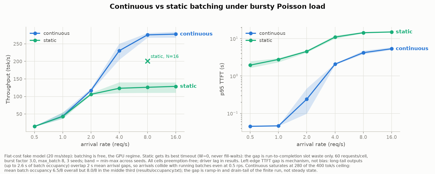
Three things worth reading off this chart:
The saturation gap is 2.15x. Continuous batching saturates around 280 tokens per second; static plateaus around 130. The theoretical ceiling is 400 (batch of 8, 20 ms steps). Continuous does not hit it because the run is finite: mean batch occupancy is 6.5 of 8 over the whole run but 8.00 of 8 in the middle third, so the gap to the ceiling is ramp-in and drain-tail, not steady-state behavior.
You cannot buy static’s way out with batch size. The x on the chart is static batching with the batch ceiling doubled to 16. Better, around 200 tokens per second, but still 30 percent below continuous running at half that ceiling. The waste is structural: a bigger batch holds more finished-and-idle slots while the longest member runs.
The arms are identical where fairness demands it. Through 2 requests per second the throughput curves match to the decimal per seed: same workload delivered, same work done. The fork starts at 4. Which makes the one place the arms differ below the fork, the TTFT panel, the interesting part.
Why idle does not save you
At 0.5 requests per second the mean gap between arrivals is 2 seconds. The output mix runs up to 128 tokens, and 128 tokens at 20 ms per step means a single long request occupies a run-to-completion batch for about 2.6 seconds. The batch is busy longer than the average gap between arrivals.
So arrivals collide with running batches even at the lightest realistic load, and they collide more often than the naive arithmetic says they should. The server was busy 29 percent of the wall clock. 56 percent of arrivals still collided with it (100 of 180 requests across three seeds). Utilization arithmetic (0.5 requests per second times the realized 0.86 s mean service time) predicts 43 percent. The extra collisions are burstiness: arrivals cluster, and a clustered arrival lands disproportionately in the shadow of the one before it. Bursty traffic oversamples busy periods, which is exactly the regime run-to-completion handles worst. A collided arrival under static batching then waits for the running batch to finish completely, however little work it has left. That is where the 2-second p95 comes from on an idle server. Continuous batching admits the same arrivals mid-flight and hands them their first token in about two step times.
The general statement: run-to-completion waste has no idle regime under a long-tailed output mix. The only way to make static batching’s tail latency match continuous is traffic so sparse that requests never overlap at all, and a server with traffic that sparse does not need a batching policy.
What this chart cannot claim
The flat-cost model means the chart demonstrates scheduling wins, not kernel wins. My engine’s real forward pass processes sequences one at a time, so it cannot show the memory-bandwidth throughput gains that compute-layer batching delivers on GPUs; that boundary is stated in the repo docs and it is why the fake model exists. The benchmark also proves it delivered its own workload: per-request schedule lag is recorded, and it held near 5 ms across every cell, orders of magnitude below any measured effect. Every cell on the chart was preemption-free by construction, so exactly one mechanism is being measured. The full results and the harness are in the repo.
One result from outside the main sweep deserves a sentence: in a separate ablation under deliberate memory pressure, the continuous arm preempted three times as often as static and still won on both throughput and tail latency. The scheduler spends preemptions freely and profits, which is early evidence that cheap preemption (abort, requeue, resume exactly) was the right design for the eviction work this engine exists to study.
What this engine is for
Continuous batching is a solved problem; this chart exists so the instrument that produced it is trustworthy. The open problem is one layer down: when GPU memory fills, which cached state do you evict, offload, or recompute? Three papers attacked that question this year with no common benchmark and no measured costs. Measuring those costs is next.